Have you ever tried to create a perfect circle or ball for your cross stitch-, crochet- or knitwork? In this article I will explain how to create a perfect 2-dimensional circle with the use of excel.
I came across the book by Alyssa Westhoek and started to randomly cross stitch a sea and beach-life scenery. Then, as a background, I wanted to create a bigger circle than Alyssa’s examples. And it also needed to be a nice and even circle…. It is very hard to create a good one without the use of any tools. If your canvas/circle is still quite small you might want to consider to bind a pencil on a rope while using graph paper. For bigger circles I found a good method by using the Excel program and with the help of my formulas and the excel sheet that you can download further below, you will be able to create a perfect circle in Excel by yourself.
Parameters of a circle
Just a bit of background on how to describe a circle with it’s parameters. These are used to further calculate dimensions from. It is not necessary to completely understand all the details of the formulas in this article but it will ease the use of the formulas in the Excel sheet further below….
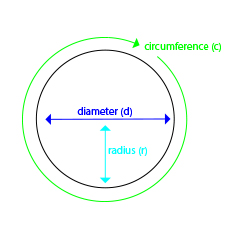
First some general parameters:
- d is the diameter
- r is the radius
- r is half of the diameter: r=1/2d
- c = the circumference= 2πr
- π= 3.14 (rounded) and is a fixed number that is used for calculations on circles
- α= angle: each circle has 360 degrees if you go round, e.g. a quarter has 90 degrees
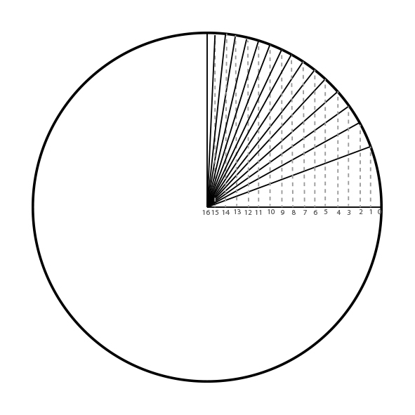
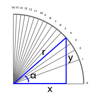
For the circle, the r always remains the same when you are on the circle. The x changes in equal steps (from 0-16) and the alpha and the y are the unknowns.
So now that we know some parameters of a circle, we will need to define how big the circle needs to be. When looking at your stitch canvas, you will work with cross-stitches per cm. For example 14ct -> 5.4 cross stitches per cm. 3 cm radius will mean 3×5.4=16,2 cross stitches in the radius, rounded off 16, so then r=16 cross stitches.
The formulas required to calculate a circle / triangles
Now we need to introduce the mathematical functions, sinus and cosinus. These functions we will require to calculate the x and the y. You will not really need to know what the background is of these functions, however these are the ones that are used in the excel formulas:
- y= sin(α) *r
- y/r=sin(α)
- x= cos(α) *r
- x/r=cos(α)
- α=acos(x/r)
Inserting the parameters and formulas into Excel
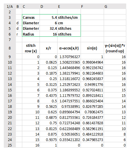
Look at the excel table, picture copied in below. You know the values in the green square, so you can fill these in. You also know how many rows you have which is the x (in this example x ranges from 0-16, and the highest number 16 is always the value of radius r) which you can fill in for fields C9-C25 (the number of rows in column c you will need to adapt to your own example, based on the radius).
Since we know the x and we know the r, we can therefore simply fill in the formulas:
- row 1, x=1; r=16 (r is the radius which is the same for each row)
- Using acos (x/r) = α = acos (1/16) = ±1,51 -> this is the angle α, see table.
- See further all calculated angles α in the table, column E.
Once you have the α for each row, you can use the formula y=sin(α)*r to calculate y, see column F. For row 1 this is y=sin(1,51)*16=±16
For calculating within Excel it means entering the following formulas into the fields:
- column D9 and further: example D9: “=C9/$D6” which means “=x/r” (the x is in column C and the r is in D6). D10: “=C10/$D6” etc etc.
- column E9 and further: “=acos(D9)” which means “=acos(x/r)” which gives us the α of D9.
- column F9 and further: “=sin(E9)” which means “=sin(α)” and this is the intermediate step to get to to calculate y for row 9.
- column G9 and further: =ROUNDUP(F9*D$6,0) which means “sin(α)*r=y round up to 0 decimals” The F9 refers to the “sin(α): that was calculated for x in F9.
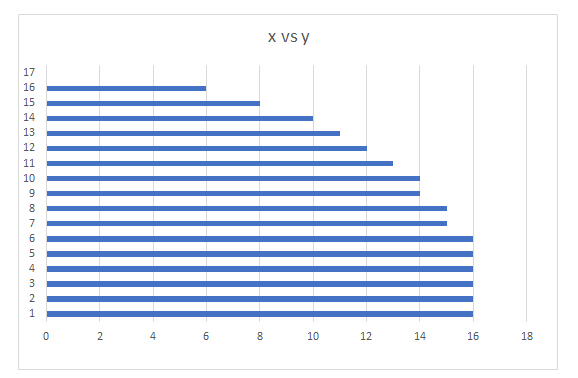
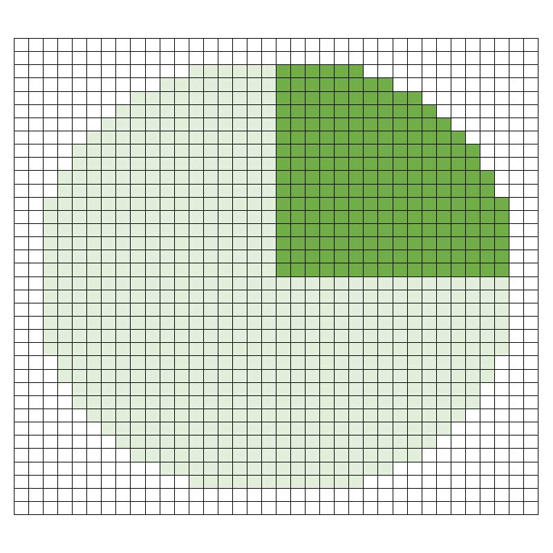
And voila: you now have in column C the x and in column G the y. This example is for a quarter of a circle and you can easily mirror it for the other quarters. The below picture is a graphical visualization of the quarter that you just calculated.